Script example of curve projection

This document shows how to use the algorithm of trajectory projection to design feasible gradient waveforms.

Run the file 'script_example_gradient_waveform.m'

Contents

Enter the Gradient constraints

close all
clear all
clc

Parameters of the scanner (here used in [Lustig et al, IEEE TMI 2008])

Gmax = 40e-3;  % T/m
Smax = 150e-3; % T/m/ms
Kmax = 600;     % m^-1

gamma = 42.576*1e3; % kHz/T

alpha = gamma*Gmax;  % in m^-1 ms^-1
beta  = gamma*Smax;  % in m^-1 ms^-2
Dt    = .004;        % sampling time in ms

Choose an input trajectory for the algorithm

Give an input trajectory

load citiesTSPexample
x=pts*Kmax;
s0=parameterize_maximum_speed(x,.8*alpha,Dt)';

figure, plot(s0(1:end,1),s0(1:end,2),'b.','linewidth',2)
axis equal, axis off
set(gcf,'Color',[1 1 1])
legend('input trajectory')

Specify constraints

dt=Dt;  % discretisation step;

% define kinematic constraints
%C_kine=set_MRI_constraints_RV(alpha,beta,dt);  % Rotation Variant Constraints
C_kine=set_MRI_constraints_RIV(alpha,beta,dt); % Rotation Invariant Constraints

% and affine constraints
C_linear=set_Linear_constraints(size(s0,1),size(s0,2));
%C_linear=set_Linear_constraints(size(s0,1),size(s0,2),'start_point',[0 0],'end_point',[0 0],'gradient_moment_nulling',1,'curve_splitting',1400);

% Algorithm parameters
Algo_param.nit = 30000;  % number of iterations
Algo_param.L=16;    % Lipschitz constant of the gradient
Algo_param.discretization_step=dt;

% optional parameters (default 0)
Algo_param.show_progression = 0; % 0 = no progression , can be really slow
Algo_param.display_results  = 1;

Project curve with Rotation-Invariant Constraints

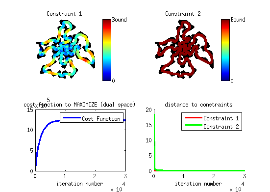
tic
s1=Project_Curve_Affine_Constraints(s0,C_kine,C_linear,Algo_param);
toc

----------------------
Constraint verifications:

Value of constraint 1: 5.9609   (Bound: 6.8122)
Value of constraint 2: 0.10596   (Bound: 0.10218)
----------------------
----------------------
Elapsed time is 75.540057 seconds.

Display the output trajectory

figure, plot(s0(:,1),s0(:,2),'b','linewidth',2)
hold on,
plot(s1(:,1),s1(:,2),'r','linewidth',3)
axis equal, axis off
set(gcf,'Color',[1 1 1])
legend('input trajectory', 'projected trajectory')

Display the gradient

g1=Prime(s1,Dt)/gamma;
gg1=Second(s1,Dt)/gamma;
T=size(s1,1);

figure,
plot(g1(:,1),'r','linewidth',3), axis([0 T*1.1 -Gmax*1.1 Gmax*1.1])
hold on, plot(g1(:,2),'b','linewidth',3), axis([0 T*1.1 -Gmax*1.1 Gmax*1.1])
g1n=sqrt(g1(:,1).^2+g1(:,2).^2);
hold on, plot(g1n,'k','linewidth',3), axis([0 T*1.1 -Gmax*1.1 Gmax*1.1])
set(gcf,'Color',[1 1 1])
hold on, plot((1:T),0*(1:T), '--k','lineWidth',3)
hold on, plot((1:T),0*(1:T)+Gmax, '--k','lineWidth',2)
hold on, plot((1:T),0*(1:T)-Gmax, '--k','lineWidth',2)
set(gca,'XTick',[0,T])
set(gca,'XTickLabel',{'0',T*Dt})
set(gca,'YTick',[-Gmax,Gmax])
set(gca,'YTickLabel',{-Gmax*1e2,Gmax*1e2})
set(gca,'FontSize',15)
ylabel('G/cm')
xlabel('ms')
hold off
h_legend=legend('$ g_x(t)$','$ g_y(t)$','$|g(t)|$');
set(h_legend,'FontSize',20,'interpreter','latex');
title('Gradient Waveforms')

figure,
plot(gg1(:,1),'r','linewidth',3), axis([0 T*1.1 -Smax*1.1 Smax*1.1])
hold on, plot(gg1(:,2),'b','linewidth',3), axis([0 T*1.1 -Smax*1.1 Smax*1.1])
gg1n=sqrt(gg1(:,1).^2+gg1(:,2).^2);
hold on, plot(gg1n,'k','linewidth',3), axis([0 T*1.1 -Smax*1.1 Smax*1.1])
set(gcf,'Color',[1 1 1])
hold on, plot((1:T),0*(1:T), '--k','lineWidth',3)
hold on, plot((1:T),0*(1:T)+Smax, '--k','lineWidth',2)
hold on, plot((1:T),0*(1:T)-Smax, '--k','lineWidth',2)
set(gca,'XTick',[0,T])
set(gca,'XTickLabel',{'0',T*Dt})
set(gca,'YTick',[-Smax,Smax])
set(gca,'YTickLabel',{-Smax*1e2,Smax*1e2})
set(gca,'FontSize',15)
ylabel('G/cm/ms')
xlabel('ms')
hold off
h_legend=legend('$ \dot g_x(t)$','$ \dot g_y(t)$','$| \dot g(t)|$');
set(h_legend,'FontSize',20,'interpreter','latex');
title('Slew rate')

Published with MATLAB® R2014a