Script example curve projection
This document shows how to use the algorithm of trajectory projection to design feasible gradient waveforms.
Contents
Enter the Gradient constraints
close all
clear all
clc
Parameters of the scanner (here used in [Lustig et al, IEEE TMI 2008])
Gmax = 40e-3;  % T/m
Smax = 150e-3; % T/m/ms
Kmax = 600;     % m^-1

gamma = 42.576*1e3; % kHz/T

alpha = gamma*Gmax;  % in m^-1 ms^-1
beta  = gamma*Smax;  % in m^-1 ms^-2
Dt    = .004;        % sampling time in ms
Choose an input trajectory for the algorithm
Give an input trajectory
load citiesTSPexample
x=pts*Kmax;
s0=parameterize_maximum_speed(x,.4*alpha,Dt)';

% w1 = 14.7*2*pi*Gmax;
% w2 = 8.7/1.02*2*pi*Gmax;
% T = .17/Gmax;
% t = 0e-3:Dt:T;
% C = Kmax*sin(w1*t').*exp(1i*w2*t');
% x=[real(C)';imag(C)'];
% s0=parameterize_maximum_speed(x,.9*alpha,Dt)';

figure, plot(s0(1:end,1),s0(1:end,2),'b.','linewidth',2)
axis equal, axis off
set(gcf,'Color',[1 1 1])
legend('input trajectory')

Specify constraints
dt=Dt;  % discretisation step;

% define kinematic constraints
C_kine=set_MRI_constraints_RV(alpha,beta,dt);  % Rotation Variant Constraints
%C_kine=set_MRI_constraints_RIV(alpha,beta,dt); % Rotation Invariant Constraints

% and affine constraints
%C_linear=set_Linear_constraints(size(s0,1),size(s0,2),'start_point',[0 0]);
C_linear=set_Linear_constraints(size(s0,1),size(s0,2),'start_point',[0 0],'end_point',[0 0],'gradient_moment_nulling',1,'curve_splitting',1400);

% Algorithm parameters
Algo_param.nit = 100000;  % number of iterations
Algo_param.L=16;    % Lipschitz constant of the gradient
Algo_param.discretization_step=dt;

% optional parameters (default 0)
Algo_param.show_progression = 0; % 0 = no progression , can be really slow
Algo_param.display_results  = 1;
Project curve with Rotation-Invariant Constraints
tic
s1=Project_Curve_Affine_Constraints(s0,C_kine,C_linear,Algo_param);
toc
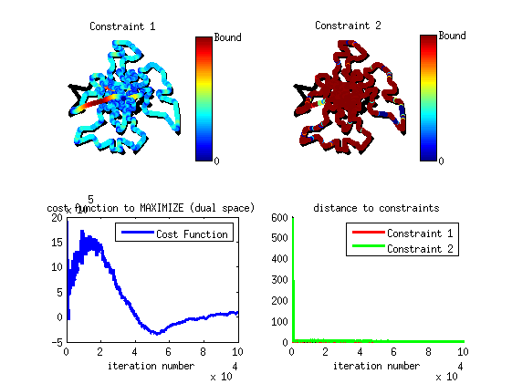
----------------------
Constraint verifications:

Value of constraint 1: 6.8982   (Bound: 6.8122)
Value of constraint 2: 0.13604   (Bound: 0.10218)
----------------------
----------------------
Elapsed time is 399.873498 seconds.
Display the output trajectory
figure, plot(s0(:,1),s0(:,2),'b','linewidth',2)
hold on,
plot(s1(:,1),s1(:,2),'r','linewidth',3)
axis equal, axis off
set(gcf,'Color',[1 1 1])
legend('input trajectory', 'projected trajectory')
